Photo by badjonni

It’s been a while since I last wrote about using eight bit for inference with deep learning, and the good news is that there has been a lot of progress, and we know a lot more than we did even a year ago. There are still a lot of unanswered questions too, which is why I’m waiting for a plane to take me to MobiSys, where I’ll be helping Nic Lane from UCL run a workshop for the research community to investigate some of them.

As a foundation for that, I’ll be giving a talk on what I know now, and what my hunches are. A lot of it is empirical, and we don’t have nearly enough rigorous experiments, let alone published papers, but if you take all this as provisional I hope it might still be useful. I’m also very happy to acknowledge my deep debt to my Google colleagues and others like Song Han who are the driving forces behind much of this work! Here are my notes on the areas I’ll be covering tomorrow.

Hardware implementations

Since the original TPU paper has been published, we can now use that as a successful example of using eight bit for inference across a wide variety of models within Google. There’s also the collaboration between the Qualcomm and TensorFlow teams that enables models to run up to seven times faster on the HVX DSP than on the CPU, thanks to the use of eight bit. This means we now have more evidence that this is a good approach to use on the hardware side.

Training with forward passes

I don’t have any published papers to hand, and we haven’t documented it well within TensorFlow, but we do have support for “fake quantization” operators. If you include these in your graphs at the points where quantization is expected to occur (for example after convolutions), then in the forward pass the float values will be rounded to the specified number of levels (typically 256) to simulate the effects of quantization. In the backward pass, this rounding won’t be performed, so gradients will be calculated using full float values. This has the effect of forcing the graph to adapt to the lower precision it will encounter during inference, and in practice we’ve seen this improve the accuracy of the quantized graph dramatically, sometimes to a level indistinguishable from float. It also gives precalculated min/max ranges for the 32-bit to 8-bit downscaling that needs to happen after many operations. This saves a step on the CPU, but for hardware implementations it’s even more important, since a dynamically-calculated range may be impossible to efficiently implement.

By the way, if you do want fixed ranges but can’t retrain, there are some options for running example data through a pretrained network to bake them in instead.

Exact zeroes are important

The current TensorFlow way of figuring out ranges just looks at the min/max of the float values and assigns those to 0 and 255. This means that real zero is almost always not exactly representable, and the closest encoded value may represent something like 0.046464, or some other arbitrary distance from exact zero. For most numbers this doesn’t matter, because the float values are assumed to occur in a ‘random’ enough way that the error on the representation of any individual value is also uniformly random. The idea is that as long as the errors generally cancel each other out, they’ll just appear as the kind of random noise that the network is trained to cope with and so not destroy the overall accuracy by introducing a bias.

The problem is that the real value of zero shows up a lot more often you’d expect in neural network calculations. Convolutions are padded with zeros at the edges when filters overlap, and the Relu activation function gates any negative numbers at zero. This means that any error in the zero representation contributes disproportionately to overall results.

The solution to this is to ensure that real values of zero are represented as exactly as possible in the quantized encoding. The way to do this is to nudge the overall min/max values so that zero is exact. We’re not (yet) doing this in TensorFlow, but hope to have it in soon. For much more information, Benoit Jacob has some excellent documentation in gemmlowp, and is the source of most of the information above.

Asymmetric ranges are inconvenient, but may be necessary

Constraining the min/max ranges so that the minimum is always the negative of the maximum is very convenient for a lot of purposes because it avoids having to apply an offset to the operands to the matrix multiply. Unfortunately the evidence for whether this allows for enough precision is mixed, with some models showing unacceptable loss of overall accuracy. This is still an open question, and an area where we need more experiments.

Excluding -128 can be useful

One practical issue that has come up in various contexts is that signed eight bit values run from -128 to +127. This is inconvenient because there’s one more value on the negative side than the positive, and so requires careful handling if we want to use symmetric ranges and ensure zero is exactly representable as encoded zero. Unrelatedly, it’s also been helpful with the ARM NEON CPU implementation to avoid -128 for the weights to allow a faster code path. There’s not all that much principle behind it yet, but there’s thus some evidence that avoiding -128 in general may be helpful.

Lower bit depths are promising, but unproven

There have been some fantastic papers around four bit, two bit, or even one bit precision for neural networks. Unfortunately so far they’ve all had some practical drawbacks that have prevented us from taking advantage of them. Song Han’s four-bit weights require a lookup table, which makes them hard to implement efficiently at runtime, though I’m intrigued to know if a simple function to handle the nonlinear distribution might work as well and be easier to optimize. We haven’t been able to achieve the accuracy we need on models we care about using lower bit depths, or even four-bit linear. The number of one-bit ops required also seems to scale in a way that negates the advantage of their lower precision. Unfortunately I don’t have any papers or documented experiments to share on this though, and I’m also hopeful that these issues can be overcome in the future, so I’ll be keeping a close eye on the literature.

Models are important

A lot of what I’m discussing above are fairly low-level optimizations, but as we know from software engineering, the biggest gains are often to be found higher up the stack. Switching to a more efficient sorting algorithm will probably do more for traditional code than rewriting a less-suited one in assembler. In the same spirit, altering the model architectures so that there’s less work to do is usually a much bigger win than tweaking the bit depth. That’s why I was very pleased that we could release the Mobilenet family of models. These substantially reduce the amount of computation needed, and also work well with quantization, thanks to hard work by Andrew Howard, Benoit Jacob, Dmitry Kalenichenko, and the rest of the Mobile Vision team.

As we keep pushing on quantization, this sort of co-design between researchers and implementers is crucial to get the best results. I think there’s a whole new field beginning to emerge, which I’m not sure whether to call ML Engineering or ML Systems, looking at the whole lifecycle of a deep learning solution, all the way from initial research through to deployment in production. It’s only with that sort of integrated view that we’re going to be able to solve some of the outstanding problems we’re still facing.

Photo by The Alien Experience

I miss having a dog, and I’d love to have a robot substitute! My friend Lukas built a $100 Raspberry Pi robot using TensorFlow to wander the house and recognize objects, and with the person detection model it can even follow me around. I want to be able to talk to my robot though, and at least have it understand simple words. To do that, I need to write a simple speech recognition example for TensorFlow.

As I looked into it, one of the biggest barriers was the lack of suitable open data sets. I need something with thousands of labelled utterances of a small set of words, from a lot of different speakers. TIDIGITS is a pretty good start, but it’s a bit small, a bit too clean, and more importantly you have to pay to download it, so it’s not great for an open source tutorial.  I like https://github.com/Jakobovski/free-spoken-digit-dataset, but it’s still small and only includes digits. LibriSpeech is large enough, but isn’t broken down into individual words, just sentences.

To solve this, I need your help! I’ve put together a website at https://open-speech-commands.appspot.com/ (now at https://aiyprojects.withgoogle.com/open_speech_recording) that asks you to speak about 100 words into the microphone, records the results, and then lets you submit the clips. I’m then hoping to release an open source data set out of these contributions, along with a TensorFlow example of a simple spoken word recognizer. The website itself is a little Flask app running on GCE, and the source code is up on github. I know it doesn’t work on iOS unfortunately, but it should work on Android devices, and any desktop machine with a microphone.

I’m hoping to get as large a variety of accents and devices as possible, since that will help the recognizer work for as many people as possible, so please do take five minutes to record your contributions if you get a chance, and share with anyone else who might be able to help!

Photo by PixelMixer

I gave a talk last week at the Embedded Vision Summit, and one question that came up was how to run neural networks trained in TensorFlow on tiny, power-efficient CPUs like the EFM32. This microcontroller is based on an ARM M4 design, and uses about 2.5 milliwatts when running at 40 MHz. It’s not much to work with, but it does at least have 256KB of RAM and 1024KB of flash program memory. This is more than enough to run some simple neural networks, especially for tasks like audio hotword detection that don’t need ultra-high accuracy to be useful. It is a tricky task though, since it requires a combination of ML and embedded hardware expertise. Here’s how I would tackle it:

Make sure you can train a model on the desktop that achieves the accuracy you need for your product, ignoring embedded constraints. Usually the hardest part here is getting enough relevant training data, since for good results you’ll need something that reflects the actual data you’ll be seeing on the device.

Once you have a proof of concept model working, try to shrink it down to fit the constraints of your device. This will involve:

• Making sure the number of weights is small enough to fit in RAM. You can compress them down to eight bit in most cases to help. The tensorflow/tools/graph_transform/summarize_graph tool will give you estimates on the number of weights.
• Reduce the size of the fully-connected and convolutional layers so that the number of compute operations is small enough to run within your device’s budget. The tensorflow/tools/benchmark utility with –show_flops will give you an estimate of this number. For example, I might guess that an M4 could do 2 MFLOPs/second, and so aim for a model that fits in that limit.

When you have a model that looks like it should fit, write a custom runtime to execute it. Right now I wouldn’t recommend using the standard TensorFlow runtime on an embedded device because the binary size overhead of a general interpreter is too large. Instead, manually write a piece of code that loads your weights and does the matrix multiplies. Usually your model will be comparatively simple, just a couple of fully-connected layers for example, so hopefully the amount of coding won’t be overwhelming. I am hoping we have a better solution and some examples for this use case in the future though, since I think it’s an area where neural network solutions are going to make a massive impact!

I’ve been very impressed by how seriously the TensorFlow team and leadership have taken supporting the open source community, so I was glad I was able to write up some of the approaches we took at O’Reilly last week. The process is definitely not perfect though, just take a look at my awful backlog of Github issues! I’m hoping we’ll be able to keep learning and improving how we do things, and I’d be interested to hear how other commercial teams handle these sort of problems too.

I’ve found collecting great data is a lot more important than using the latest architecture when you’re trying to get good results in deep learning, so ever since my Jetpac days I’ve spent a lot of time trying to come up with good ways to refine my training sets. I’ve written or used a lot of different user interfaces custom designed for this, but surprisingly I’ve found that the stock Finder window in OS X has been the most productive!

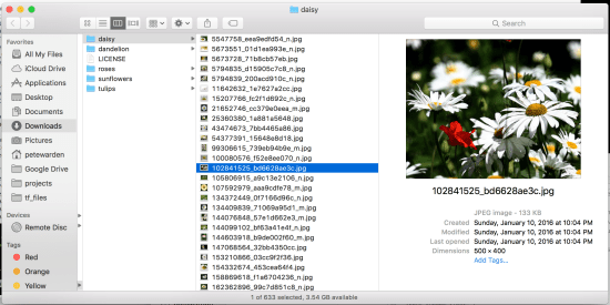
Here is how I curated the flowers set of images that’s used in TensorFlow for Poets, and I’ve found I can sort through many thousands of images an hour using this approach.

• Copy and decompress the images onto a folder on my OS X machine.
• Open the folder in the OS X Finder app, the normal file viewer.
• Choose the ‘Column’ view for the Finder window, which is an icon in the top bar, the third from the left in the view choices.
• Select the first image. You should now see a small preview picture in the right-hand column.
• Move the mouse pointer over the right-hand edge of the window, until you see the cursor change into a ‘drag left/right’ icon.
• Drag the right-hand side of the Finder window out. You should see the image preview get larger. Stop once the preview size is no longer growing.

You should now have a window that looks like the image at the start of the post. There are a couple of ways of using this view. If I have a set of images that have been roughly sorted, but I want to do some quality control by weeding out pictures that are misclassified, I’ll use the up and down arrow keys to move through the images, look at each preview to quickly tell if it’s correct, and press the Command and Delete keys to remove it if not. After removing a photo, the selection automatically moves onto the next image, which is convenient.

If I have a large set of photos I want to label as belonging to a set of categories, rather than just rejecting bad labels, then I’ll use a slightly more involved approach. The key is to use “Tags” in OS X (which used to be called labels). You can follow these instructions for setting up a keyboard shortcut to open the Tags menu for an item, and then move through the files using the down keys, assigning tags as you go. Unfortunately OS X removed the ability to apply particular tags through a single keyboard shortcut, which used to be possible in older versions of the system, but this can still be an efficient way to label large sets of images.

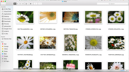
Another approach I sometimes use to very quickly remove a small number of bad labels is to open a folder of images using the Icon view in the finder, and then crank up the preview size slider in the bottom right corner of the window. You may have to select “View->Arrange By->Name” from the top menu to ensure that the enlarged icons all fit inside the window.

I don’t find this as efficient for moving through every image as the column view, but if I want to quickly visually scan to find a few rogue images it’s very handy. I’ll usually just grab the scroll bar at the right hand side, or use mouse scroll to quickly look through the entire data set, and then click to select any that I want to remove.

What I like about these approaches are that they are very lightweight, I don’t need to install any special software, and the speed of the preview loading in the Finder beats any custom software that I’ve found, so I can run through a lot of images very fast. Anyway, I hope you find them useful too, and do let me know your favorite labeling hacks in the comments or on Twitter.

Photo by Daniel Lopez

Take a look at this function:

 for (j = 0; j < n; j++) {
   for (i = 0; i < m; i++) {
     float total(0);
     for (l = 0; l < k; l++) {
       const size_t a_index = ((i * a_i_stride) + (l * a_l_stride));
       const float a_value = a[a_index];
       const size_t b_index = ((j * b_j_stride) + (l * b_l_stride));
       const float b_value = b[b_index];
       total += (a_value * b_value);
     }
     const size_t c_index = ((i * c_i_stride) + (j * c_j_stride));
     c[c_index] = total;
   }
 }

For something so simple, it turns out it’s amazingly hard for compilers to speed up without a lot of human intervention. This is the heart of the GEMM matrix multiply function, which powers deep learning, and every fast implementation I know has come from old-school assembler jockeys hand-tweaking instructions!

When I first started looking at the engineering side of neural networks, I assumed that I’d be following the path I’d taken on the rest of my career and getting most of my performance wins from improving the algorithms, writing clean code, and generally getting out of the way so the compiler could do its job of optimizing it. Instead I spend a large amount of my time worrying about instruction dependencies and all the other hardware details that we were supposed to be able to escape in the 21st century. Why is this?

Matrix multiplies are a hard case for modern compilers to handle. The inputs used for neural networks mean that one function call may require millions of operations to complete, which magnifies the latency impact of any small changes to the code. The access patterns are entirely predictable for a long period, but not purely linear, which doesn’t fit well with cache line algorithms as written in the naive way above. There are lots of choices about how to accumulate intermediate results and reuse memory reads, which will have different outcomes depending on the sizes of the matrices involved.

All this means that an endangered species, hand-coding assembler experts, write all of the best implementations. GotoBlas (which evolved into OpenBlas) showed how much speed could be gained on Intel CPUs. Eigen has had a lot of work put into it to run well on both x86 and ARM with float, and gemmlowp is optimized for eight-bit on ARM. Even if you’re running on a GPU, Scott Gray (formerly at Nervana, now at OpenAI) has shown how much faster hand-coded solutions can be.

This is important because it means that there’s a lot of work involved in getting good performance from new platforms, and there’s often a big gap between existing highly-optimized solutions and those ported from other architectures. This is visible for example with gemmlowp on x86, where the hand optimization is still a work in progress and so the speed still lags behind float alternatives right now.

It’s also exciting, because the real-world performance of even most optimized libraries lags behind the theoretical limits of the hardware, so there are still opportunities to squeeze more speed out of them with some clever hacking. There are also exciting developments in fundamentally different approaches to the problem like the Winograd algorithm. The good news is that if you’re an old-school assembler hacker there’s still an important place for you in the brave new world of deep learning, so I hope we can pull you in!

Photo by Stephen D. Strowes

One of the most interesting things about neural networks for me is that they’re programs you can do meaningful computation on. The most obvious example of that is automatic differentiation, but even after you’ve trained a model there are lots of other interesting transformations you can apply. These can be as simple as trimming parts of the graph that aren’t needed for just running inference, all the way to folding batch normalization nodes into precalculated weights, turning constant sub expressions into single nodes, or rewriting calculations in eight bit.

Many of these operations have been available as piecemeal Python scripts inside the TensorFlow codebase, but I’ve spent some time rewriting them into what I hope is a much cleaner and easier to extend C++ Graph Transform Tool. As well as a set of predefined operations based on what we commonly need ourselves, I’ve tried to create a simple set of matching operators and other utilities to encourage contributors to create and share their own rewriting passes.

I think there’s a lot of potential for computing on compute graphs, so I’m excited to hear what you can come up with! Do cc me (@petewarden) on github too with any issues you encounter.

Picture by Torley

A few months ago I returned to my home town of Cambridge to attend the first ARM Research Summit. What was special about this conference was that it focused on introducing external researchers to each other, rather than pushing ARM’s own agenda. They had invited a broad range of people they worked with, from academic researchers to driver engineers, and all we had in common was that we spent a lot of time working on the ARM platform. This turned out fantastically for me at least, because it meant I had the chance to learn from experts in fields I knew nothing about. As such, it left my mind spinning a little, and so this post is a bit unusual! I’m trying to clarify gut feelings about the future with some actual evidence, so please bear with me as I work through my reasoning.

One of my favorite talks was on energy harvesting by James Myers. This table leapt out at me (apologies to James if I copied any of his figures incorrectly):

Energy harvesting rules of thumb:

• Human vibration – 4µW/cm2
• Industrial vibration – 100µW/cm2
• Human temperature difference – 25µW/cm2
• Industrial temperature difference – 1 to 10 mW/cm2
• Indoor light – 10µW/cm2
• Outdoor light – 10mW/cm2
• GSM RF – 0.1µW/cm2
• Wifi RF – 0.001µW/cm2

What this means in plain English is that you can expect to harvest four micro-watts (millionths of a watt or µW) for every square centimeter of a device relying on human vibration. A solar panel in sunlight could gather ten milliwatts (thousandths of a watt or mW) for every square centimeter. If you think about an old incandescent bulb, that burns forty watts, and even a modern cell phone probably uses a watt or so when it’s being actively used, so the power you can get from energy harvesting is clearly not enough for most applications. My previous post on smartphone energy consumption shows that even running an accelerometer takes over one twenty milliwatts, so clearly it’s hard to build devices that rely on these levels of power.

Why does that matter? I’m convinced that smart sensors are going to be massively important in the future, and that vision can’t work if they require batteries. I believe that we’ll be throwing tiny cheap devices up in the air like confetti to scatter around all the environments we care about, and they’ll result in a world we can intelligently interact with in unprecedented ways. Imagine knowing exactly where pests are in a crop field so that a robot can manually remove them rather than indiscriminately spraying pesticides, or having stickers on every piece of machinery in a factory that listen to the sounds and report when something needs maintenance.

These sort of applications will only work if the devices can last for years unattended. We can already build tiny chips that do these sort of things, but we can’t build batteries that can power them for anywhere near that long, and that’s unlikely to change soon.

Can the cloud come to our rescue? I’m a software guy, but everything I see in the hardware world shows that transmitting signals continuously takes a lot of energy. Even with a protocol like BLE sending data just a foot draws more than 10 milliwatts. There seems to be an enduring relationship between power usage and the distance you’re sending the data, with register access cheaper than SRAM, which is far cheaper than DRAM, which beats radio transmission.

That’s why I believe our only hope for long-lived smart sensors is driving down the energy used by local compute to the point at which harvesting gives enough power to run useful applications. The good news is that existing hardware like DSPs can perform a multiply-add for just low double-digit picojoules, and can access local SRAM to avoid the costs of DRAM. If you do the back of the envelope calculations, a small image network like Inception V1 takes about 1.5 billion multiply-adds, so 20 picojoules * 1.5 billion gives a rough energy cost of 30 millijoules per prediction (or 30 milliwatts at 1 prediction per second). This is already an order of magnitude less energy than the equivalent work done on a general-purpose CPU, so it’s a good proof that it’s possible to dramatically reduce computational costs, even though it’s still too high for energy harvesting to work.

That’s where another recurrent theme of the ARM research conference started to seem very relevant. I didn’t realize how much of a problem keeping results reliable is as the components continue to shrink. Increasingly large parts of the design are devoted to avoiding problems like Rowhammer, where accesses to adjacent DRAM rows can flip bits, as Onur Mutlu explained. It’s not just memory that faces problems like these, CPUs also need to be over-engineered to avoid errors introduced by current leakage and weirder quantum-level effects.

I was actually very excited when I learned this, because one of the great properties of neural networks is that they’re very resilient in the face of random noise. If we’re going to be leaving an increasing amount of performance on the table to preserve absolute reliability for traditional computing applications, that opens the door for specialized hardware without those guarantees that will be able to offer increasingly better energy consumption. Again, I’m a software engineer so I don’t know exactly what kinds of designs are possible, but I’m hoping that by relaxing constraints on the hardware the chip creators will be able to come up with order-of-magnitude improvements, based on what I heard at the conference.

If we can drive computational energy costs down into the femtojoules per multiply-add, then the world of ambient sensors will explode. As I was writing, I ran across a new startup that’s using deep learning and microphones to predict problems with machinery, but just imagine when those, along with seismic, fire, and all sorts of other sensors are scattered everywhere, too simple to record data but smart enough to alert people when special conditions occur. I can’t wait to see how this process unfolds, but I’m betting unreliable electronics will be a key factor in making it possible.

In TensorFlow for Poets, I showed how you could train a neural network to recognize objects using your own custom images. The next step is getting that model into users’ hands, so in this tutorial I’ll show you what you need to do to run it in your own iOS application.

I’m assuming you’ve already completed TensorFlow for Poets, and so you should have Docker installed and a tf_files folder in your home directory that contains a retrained_graph.pb file containing your model. If you don’t, you’ll need to work through that example to build your own network.

You’ll find the screencast to accompany this tutorial above, or at https://www.youtube.com/watch?v=_bkZPpniYdo, which should help clarify the steps I’ll be walking you through.

As a first step, open the Docker QuickStart Terminal and start a new docker container using the latest Docker image. This tutorial relies on some newer features of TensorFlow, so the v0.8 image used for the original TF for Poets won’t work.

docker run -it -p 8888:8888 -v $HOME/tf_files:/tf_files \
tensorflow/tensorflow:nightly-devel

You should find yourself in a new shell where the prompt begins with root@ and ends with a ‘#’, indicating you’re running inside the Docker image. To make sure things are setup correctly, run this `ls -lah /tf_files/` and make sure that the retrained_graph.pb file appears.

Next, we’re going to make sure that the model is producing sane results at the start. Here I’m using the default flower images to test, but if you have trained on custom categories substitute the image file with one of your own. The compilation process may take a few minutes too, so make sure that you have updated the VirtualBox settings to take advantage of your machine’s memory and processors if things are running too slowly.

cd /tensorflow/
bazel build tensorflow/examples/label_image:label_image
bazel-bin/tensorflow/examples/label_image/label_image \
--output_layer=final_result \
--labels=/tf_files/retrained_labels.txt \
--image=/tf_files/flower_photos/daisy/5547758_eea9edfd54_n.jpg \
--graph=/tf_files/retrained_graph.pb

This should hopefully produce a sensible top label for your example, in the case of flowers with daisy at the top. We’ll be using this command to make sure we’re still getting sensible results as we do further processing on the model file to prepare it for use in a mobile app.

Mobile devices have limited amounts of memory, and apps need to be downloaded, so by default the iOS version of TensorFlow only includes support for operations that are common in inference and don’t have large external dependencies. You can see the list of supported ops in the tensorflow/contrib/makefile/tf_op_files.txt file. One of the operations that isn’t supported is DecodeJpeg, because the current implementation relies on libjpeg which is painful to support on iOS and would increase the binary footprint. While we could write a new implementation that uses iOS’s native image libraries, for most mobile applications we don’t need to decode JPEGs because we’re dealing directly with camera image buffers.

Unfortunately the Inception model we based our retraining on includes a DecodeJpeg operation. We normally bypass this by directly feeding the Mul node that occurs after the decode, but on platforms that don’t support the operation you’ll see an error when the graph is loaded, even if the op is never called. To avoid this, the optimize_for_inference script removes all nodes that aren’t needed for a given set of input and output nodes.

The script also does a few other optimizations that help speed, such as merging explicit batch normalization ops into the convolutional weights to reduce the number of calculations. Here’s how you run it:

bazel build tensorflow/python/tools:optimize_for_inference
bazel-bin/tensorflow/python/tools/optimize_for_inference \
--input=/tf_files/retrained_graph.pb \
--output=/tf_files/optimized_graph.pb \
--input_names=Mul \
--output_names=final_result

This creates a new file at /tf_files/optimized_graph.pb. To check that it hasn’t altered the output of the network, run label_image again on the updated model:

bazel-bin/tensorflow/examples/label_image/label_image \
--output_layer=final_result \
--labels=/tf_files/retrained_labels.txt \
--image=/tf_files/flower_photos/daisy/5547758_eea9edfd54_n.jpg \
--graph=/tf_files/optimized_graph.pb

You should see very similar results to the first time you ran label_image, since the underlying mathematical results should be preserved through the changes made to streamline it.

The retrained model is still 87MB in size at this point, and that guarantees a large download size for any app that includes it. There are lots of ways to reduce download sizes, and I’ll cover those in more detail in other documentation, but there’s one very simple approach that’s a big help without adding much complexity. Because Apple distributes apps in .ipa packages, all of the assets are compressed using zip. Usually models don’t compress well because the weights are all slightly different floating point values. You can achieve much better compression just by rounding all the weights within a particular constant to 256 levels though, while still leaving them in floating-point format. This gives a lot more repetition for the compression algorithm to take advantage of, but doesn’t require any new operators and only reduces the precision by a small amount (typically less than a 1% drop in precision). Here’s how you call the quantize_graph script to apply these changes:

bazel build tensorflow/tools/quantization:quantize_graph
bazel-bin/tensorflow/tools/quantization/quantize_graph \
--input=/tf_files/optimized_graph.pb \
--output=/tf_files/rounded_graph.pb \
--output_node_names=final_result \
--mode=weights_rounded

If you look on disk, the raw size of the rounded_graph.pb file is the same at 87MB, but if you right-click on it in the finder and choose “Compress”, you should see it results in a file that’s only about 24MB or so. That reflects what size increase you’d actually see in a compressed .ipa on iOS, or an .apk on Android.

To verify that the model is still working, run label_image again:

bazel-bin/tensorflow/examples/label_image/label_image \
--output_layer=final_result \
--labels=/tf_files/retrained_labels.txt \
--image=/tf_files/flower_photos/daisy/5547758_eea9edfd54_n.jpg \
--graph=/tf_files/rounded_graph.pb

This time, I would expect that the results may have slightly more noticeable changes thanks to the effects of the quantization, but the overall size and order of the labels should still be the same.

The final processing step we need to run is memory mapping. Because the buffers holding the model weight values are 87MB in size, the memory needed to load these into the app can put a lot of pressure on RAM in iOS even before the model is run. This can lead to stability problems as the OS can unpredictably kill apps that use too much memory. Fortunately these buffers are read-only, so it’s possible to map them into memory in a way that the OS can easily discard them behind the scenes when there’s memory pressure, avoiding the possibility of those crashes.

To support this, we need to rearrange the model so that the weights are held in sections that can be easily loaded separately from the main GraphDef, though they’re all still in one file. Here is the command to do that:

bazel build tensorflow/contrib/util:convert_graphdef_memmapped_format
bazel-bin/tensorflow/contrib/util/convert_graphdef_memmapped_format \
--in_graph=/tf_files/rounded_graph.pb \
--out_graph=/tf_files/mmapped_graph.pb

One thing to watch out for is that the file on disk is no longer a plain GraphDef protobuf, so if you try loading it into a program like label_image that expects one, you’ll see errors. You need to load the model file slightly differently, which we’ll show in the iOS example below.

So far we’ve been running all these scripts in Docker, since for demonstration purposes it’s a lot easier to run scripts there, because installing the Python dependencies is a lot more straightforward on Ubuntu than OS X. Now we’re going to switch to a native terminal so that we can compile an iOS app that uses the model you’ve trained.

You’ll need Xcode 7.3 or later with the command line tools installed to build the app, which you can download from Apple. You’ll also need brew, and automake to run the build script. To install it using brew, run this command:

brew install automake

Once you have those, open up a new terminal window, download the TensorFlow source (using `git clone https://github.com/tensorflow/tensorflow`) to a folder on your machine (replacing `~/projects/tensorflow` below with that location) and run the following commands to build the framework and copy your model files over:

cd ~/projects/tensorflow
tensorflow/contrib/makefile/build_all_ios.sh
cp ~/tf_files/mmapped_graph.pb \
tensorflow/contrib/ios_examples/camera/data/
cp ~/tf_files/retrained_labels.txt \
tensorflow/contrib/ios_examples/camera/data/
open tensorflow/contrib/ios_examples/camera/camera_example.xcodeproj

Check the terminal to make sure that your compilation succeeded without errors, and then you should find the camera example project opened in Xcode. This app shows a live feed of your camera, together with the labels for any objects it has recognized, so it’s a good demo project for testing out a new model.

The terminal commands above should have copied the model files you need into the apps data folder, but you still need to let Xcode know that it should include them in the app. To remove the default model files, go to the left-hand project navigator pane in Xcode, select imagenet_comp_graph_label_strings.txt and tensorflow_inception_graph.pb in the data folder, and delete them, choosing “Move to Trash” when prompted.

Next, open a Finder window containing the new model files, for example from the terminal like this:

open tensorflow/contrib/ios_examples/camera/data

Drag `mmapped_graph.pb` and `retrained_labels.txt` from that Finder window, into the data folder in the project navigator. Make sure the “Add to Targets” is enabled for CameraExample in the dialog’s checkbox. This should let Xcode know that it should include the files when you build the app, so if you see later errors about missing files, double-check these steps.

We’ve got the files in the app, but we also need to update some other information. We need to update the name of the files to load, but also some other metadata about the size of the input images, the node names, and how to scale the pixel values numerically before feeding them in. To make those changes open CameraExampleViewController.mm in Xcode, and look for the model settings near the top of the file. Replace them with the following block:

// If you have your own model, modify this to the file name, and make sure
// you've added the file to your app resources too.
static NSString* model_file_name = @"mmapped_graph";
static NSString* model_file_type = @"pb";
// This controls whether we'll be loading a plain GraphDef proto, or a
// file created by the convert_graphdef_memmapped_format utility that wraps a
// GraphDef and parameter file that can be mapped into memory from file to
// reduce overall memory usage.
const bool model_uses_memory_mapping = true;
// If you have your own model, point this to the labels file.
static NSString* labels_file_name = @"retrained_labels";
static NSString* labels_file_type = @"txt";
// These dimensions need to match those the model was trained with.
const int wanted_input_width = 299;
const int wanted_input_height = 299;
const int wanted_input_channels = 3;
const float input_mean = 128.0f;
const float input_std = 128.0f;
const std::string input_layer_name = "Mul";
const std::string output_layer_name = "final_result";

Finally, plug in and select your iOS device (this won’t run on the simulator because it needs a camera) and hit Command+R to build and run the modified example. If everything has worked, you should see the app start, display the live camera feed, and begin showing labels from your training categories.

To test it out, find an example of the kind of objects you’re trying to recognize, point the camera at it and see if it is able to give it the right label. If you don’t have any physical objects handy, try doing an image search on the web, and then point it at your computer display. Congratulations, you’ve managed to train your own model and run it on a phone!

As next steps, a lot of the same transformations can be used on Android or for the Raspberry Pi, and for all sorts of other models available in TensorFlow for everything from natural language processing to speech synthesis. I’m excited to see new apps emerge using the incredible capabilities of deep learning on device, so I can’t wait to see what you come up with!

Photo by Mark, Vicki, Ellaura, and Mason

A good friend of mine just asked me “What are GPUs?”. It came up because she’s a great digital artist who’s getting into VR, and the general advice she gets is “Buy a PC with a video card that costs more than $350”. What makes that one component cost so much, why do we need them, and what do they do? To help answer that, I thought I’d try to give an overview aimed at non-engineers.

Graphics Processing Units were created to draw images, text, and geometry onto the screen. This means they’re designed very differently than the CPUs that run applications. CPUs need to be good at following very complex recipes of instructions so they can deal with all sorts of user inputs and switch between tasks rapidly. GPUs are much more specialized. They only need to do a limited range of things, but each job they’re given can involve touching millions of memory locations in one go.

To see the difference between the kind of programs that run on CPUs and GPUs, think about a CPU reading from a text box. The CPU will sit waiting for you to press a key, and as soon as you do it might need to look in a list to figure out if there’s an autocomplete entry, check the spelling, or move to the next box if you hit return. This is a complex set of instructions with a lot of decisions involved.

By contrast, a typical GPU task would be drawing an image on-screen. A picture that’s 1,000 pixels wide and high has a million elements, and drawing it means moving all of those into the screen buffer. That’s a lot more work than just waiting for a key press, but it also involves a lot fewer decisions since you just need to move a large number of pixels from one place to another.

The differences in the kinds of tasks that CPUs and GPUs need to do means that they’re designed in very different ways. CPUs are very flexible and able to do a lot of complicated tasks involving decision-making. GPUs are less adaptable but can operate on large numbers of elements at once, so they can perform many operations much faster.

The way GPUs achieve this flexibility is that they break their tasks into much smaller components that can be shared across a large set of many small processors running at once. Because the jobs they’re being asked to do are simpler than CPUs, it’s easy to automatically split them up like this. As an example you can imagine having hundreds of little processors, each of which is given a tile of an image to draw. By having them work in parallel, the whole picture can be drawn much faster.

The key advantage of GPUs is this scalability. They can’t do every job, but for the ones they can tackle, you essentially can just pack in more processors on the board to get faster performance. This is why video cards that are capable of handling the high resolutions and framerates you need for VR are more expensive, they have more (and individually faster) processors to handle those larger sizes as you go up in price. This scalability is harder to do on CPUs because it’s much trickier to break up the logic needed to run applications into smaller jobs.

This is a painfully simplified explanation I know, but I’m hoping to get across what makes GPUs fundamentally different from CPUs. If you have a task that involves a lot of computation but few decision points, then GPUs are set up to parallelize that job automatically. This is clearest in graphics, but also comes up as part of deep learning, where there are similar heavy-lifting requirements across millions of artificial neurons. As Moore’s Law continues to fade, leaving CPU speeds to languish, these sort of parallel approaches will become more and more attractive.