Photo by Mark, Vicki, Ellaura, and Mason

A good friend of mine just asked me “What are GPUs?”. It came up because she’s a great digital artist who’s getting into VR, and the general advice she gets is “Buy a PC with a video card that costs more than $350”. What makes that one component cost so much, why do we need them, and what do they do? To help answer that, I thought I’d try to give an overview aimed at non-engineers.

Graphics Processing Units were created to draw images, text, and geometry onto the screen. This means they’re designed very differently than the CPUs that run applications. CPUs need to be good at following very complex recipes of instructions so they can deal with all sorts of user inputs and switch between tasks rapidly. GPUs are much more specialized. They only need to do a limited range of things, but each job they’re given can involve touching millions of memory locations in one go.

To see the difference between the kind of programs that run on CPUs and GPUs, think about a CPU reading from a text box. The CPU will sit waiting for you to press a key, and as soon as you do it might need to look in a list to figure out if there’s an autocomplete entry, check the spelling, or move to the next box if you hit return. This is a complex set of instructions with a lot of decisions involved.

By contrast, a typical GPU task would be drawing an image on-screen. A picture that’s 1,000 pixels wide and high has a million elements, and drawing it means moving all of those into the screen buffer. That’s a lot more work than just waiting for a key press, but it also involves a lot fewer decisions since you just need to move a large number of pixels from one place to another.

The differences in the kinds of tasks that CPUs and GPUs need to do means that they’re designed in very different ways. CPUs are very flexible and able to do a lot of complicated tasks involving decision-making. GPUs are less adaptable but can operate on large numbers of elements at once, so they can perform many operations much faster.

The way GPUs achieve this flexibility is that they break their tasks into much smaller components that can be shared across a large set of many small processors running at once. Because the jobs they’re being asked to do are simpler than CPUs, it’s easy to automatically split them up like this. As an example you can imagine having hundreds of little processors, each of which is given a tile of an image to draw. By having them work in parallel, the whole picture can be drawn much faster.

The key advantage of GPUs is this scalability. They can’t do every job, but for the ones they can tackle, you essentially can just pack in more processors on the board to get faster performance. This is why video cards that are capable of handling the high resolutions and framerates you need for VR are more expensive, they have more (and individually faster) processors to handle those larger sizes as you go up in price. This scalability is harder to do on CPUs because it’s much trickier to break up the logic needed to run applications into smaller jobs.

This is a painfully simplified explanation I know, but I’m hoping to get across what makes GPUs fundamentally different from CPUs. If you have a task that involves a lot of computation but few decision points, then GPUs are set up to parallelize that job automatically. This is clearest in graphics, but also comes up as part of deep learning, where there are similar heavy-lifting requirements across millions of artificial neurons. As Moore’s Law continues to fade, leaving CPU speeds to languish, these sort of parallel approaches will become more and more attractive.

When I talk to people outside of Google and the subject turns to neural networks I often encounter a lot of skepticism. Anybody who’s been alive over the past two decades has seen a lot of technological fads appear in an explosion of hype and fade away without making much of a lasting impact. Remember fuzzy logic, CORBA, or the Semantic Web?

Deep learning is different, and I believe this fervently because is that I’ve seen the approach deliver record-beating results in practical applications across an amazing variety of different problems. That’s why TensorFlow is so important to me personally, because it’s a great platform to share some very down-to-earth tools that demonstrate convincingly how powerful the technique can be. That’s a big reason I’ve tried to build approachable tutorials for common needs like image recognition, so everyone has a chance to see it working for themselves.

It’s also why I was over the moon to see another Google research team release Parsey McParseface! This is a state of the art sentence parser that’s built using TensorFlow. That might sound a bit esoteric, but parsing is one of the fundamental problems that computers need to tackle to understand written language. With this available, I’m starting to dream up all sorts of interesting applications I wouldn’t have been able to think about before. For instance I’d love to know what verbs and adjectives are most commonly applied to men and women in all sorts of different contexts. To illustrate my point, here’s a paragraph from a great article on why bossy is so gendered:

Finally, the most flexible approach is one that is much more labor intensive. It involves gathering a random sample of instances of bossy and then simply reading through all of them with our own eyes to determine who is being labelled bossy. This is the approach I took in my recent blog post. Because of the amount of time involved, I looked at far fewer examples than any of the approaches I’ve discussed, but I also was able to classify instances that the above approaches would have missed. The graph below illustrates what I found, namely that bossy was applied to women and girls three times more frequently than it was to men and boys. … You might think to yourself, “But there’s only 101 examples! That’s so few!”

This kind of attribution of an adjective to a subject is something an accurate parser can do automatically. Rather than laboriously going through just a hundred examples, it’s easy to set up the Parser McParseface and run through millions of sentences. The parser isn’t perfect, but at 94% accuracy on one metric, it’s pretty close to humans who get 96%.

Even better, having the computer do the heavy lifting means that it’s possible to explore many other relationships in the data, to uncover all sorts of unknown statistical relationships in the language we use. There’s bound to be other words that are skewed in similar or opposite ways to ‘bossy’, and I’d love to know what they are!

That’s just one example though. The reason I’m so excited about deep learning is that I can’t even imagine all the applications that have now become possible. Download Parser McParseface yourself and give it a try on a problem you care about, I’d love to see what you come up with!

Picture by Jaebum Joo

I’m pleased to say that we’ve been able to release a first version of TensorFlow’s quantized eight bit support. I was pushing hard to get it in before the Embedded Vision Summit, because it’s especially important for low-power and mobile devices, so it’s exciting to get it out there. All this documentation will be appearing on the main TensorFlow site also, but since I’ve talked so much about why eight-bit is important here, I wanted to give an overview of what we’ve released in this post too.

When modern neural networks were being developed, the biggest challenge was getting them to work at all! That meant that accuracy and speed during training were the top priorities. Using floating point arithmetic was the easiest way to preserve accuracy, and GPUs were well-equipped to accelerate those calculations, so it’s natural that not much attention was paid to other numerical formats.

These days, we actually have a lot of models being being deployed in commercial applications. The computation demands of training grow with the number of researchers, but the cycles needed for inference expand in proportion to users. That means pure inference efficiency has become a burning issue for a lot of teams.

That is where quantization comes in. It’s an umbrella term that covers a lot of different techniques to store numbers and perform calculations on them in more compact formats than 32-bit floating point. I am going to focus on eight-bit fixed point, for reasons I’ll go into more detail on later.

Why does Quantization Work?

Training neural networks is done by applying many tiny nudges to the weights, and these small increments typically need floating point precision to work (though there are research efforts to use quantized representations here too).

Taking a pre-trained model and running inference is very different. One of the magical qualities of deep networks is that they tend to cope very well with high levels of noise in their inputs. If you think about recognizing an object in a photo you’ve just taken, the network has to ignore all the CCD noise, lighting changes, and other non-essential differences between it and the training examples it’s seen before, and focus on the important similarities instead. This ability means that they seem to treat low-precision calculations as just another source of noise, and still produce accurate results even with numerical formats that hold less information.

Why Quantize?

Neural network models can take up a lot of space on disk, with the original AlexNet being over 200 MB in float format for example. Almost all of that size is taken up with the weights for the neural connections, since there are often many millions of these in a single model. Because they’re all slightly different floating point numbers, simple compression formats like zip don’t compress them well. They are arranged in large layers though, and within each layer the weights tend to be normally distributed within a certain range, for example -3.0 to 6.0.

The simplest motivation for quantization is to shrink file sizes by storing the min and max for each layer, and then compressing each float value to an eight-bit integer representing the closest real number in a linear set of 256 within the range. For example with the -3.0 to 6.0 range, a 0 byte would represent -3.0, a 255 would stand for 6.0, and 128 would represent about 1.5. I’ll go into the exact calculations later, since there’s some subtleties, but this means you can get the benefit of a file on disk that’s shrunk by 75%, and then convert back to float after loading so that your existing floating-point code can work without any changes.

Another reason to quantize is to reduce the computational resources you need to do the inference calculations, by running them entirely with eight-bit inputs and outputs. This is a lot more difficult since it requires changes everywhere you do calculations, but offers a lot of potential rewards. Fetching eight-bit values only requires 25% of the memory bandwidth of floats, so you’ll make much better use of caches and avoid bottlenecking on RAM access. You can also typically use SIMD operations that do many more operations per clock cycle. In some case you’ll have a DSP chip available that can accelerate eight-bit calculations too, which can offer a lot of advantages.

Moving calculations over to eight bit will help you run your models faster, and use less power (which is especially important on mobile devices). It also opens the door to a lot of embedded systems that can’t run floating point code efficiently, so it can enable a lot of applications in the IoT world.

Why Not Train in Lower Precision Directly?

There have been some experiments training at lower bit depths, but the results seem to indicate that you need higher than eight bit to handle the back propagation and gradients. That makes implementing the training more complicated, and so starting with inference made sense. We also already have a lot of float models already that we use and know well, so being able to convert them directly is very convenient.

How Can You Quantize Your Models?

TensorFlow has production-grade support for eight-bit calculations built it. It also has a process for converting many models trained in floating-point over to equivalent graphs using quantized calculations for inference. For example, here’s how you can translate the latest GoogLeNet model into a version that uses eight-bit computations:

curl http://download.tensorflow.org/models/image/imagenet/inception-2015-12-05.tgz -o /tmp/inceptionv3.tgz
tar xzf /tmp/inceptionv3.tgz -C /tmp/
bazel build tensorflow/contrib/quantization/tools:quantize_graph
bazel-bin/tensorflow/contrib/quantization/tools/quantize_graph \
--input=/tmp/classify_image_graph_def.pb \
--output_node_names="softmax" --output=/tmp/quantized_graph.pb \
--mode=eightbit

This will produce a new model that runs the same operations as the original, but with eight bit calculations internally, and all weights quantized as well. If you look at the file size, you’ll see it’s about a quarter of the original (23MB versus 91MB). You can still run this model using exactly the same inputs and outputs though, and you should get equivalent results. Here’s an example:

bazel build tensorflow/examples/label_image:label_image
bazel-bin/tensorflow/examples/label_image/label_image \
--input_graph=/tmp/quantized_graph.pb \
--input_width=299 \
--input_height=299 \
--mean_value=128 \
--std_value=128 \
--input_layer_name="Mul:0" \
--output_layer_name="softmax:0"

You’ll see that this runs the newly-quantized graph, and outputs a very similar answer to the original.

You can run the same process on your own models saved out as GraphDefs, with the input and output names adapted to those your network requires. I recommend that you run them through the freeze_graph script first, to convert checkpoints into constants stored in the file.

How Does the Quantization Process Work?

We’ve implemented quantization by writing equivalent eight-bit versions of operations that are commonly used during inference. These include convolution, matrix multiplication, activation functions, pooling operations and concatenation. The conversion script first replaces all the individual ops it knows about with quantized equivalents. These are small sub-graphs that have conversion functions before and after to move the data between float and eight-bit. Below is an example of what they look like. First here’s the original Relu operation, with float inputs and outputs:

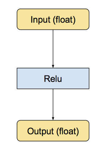
Then, this is the equivalent converted subgraph, still with float inputs and outputs, but with internal conversions so the calculations are done in eight bit.

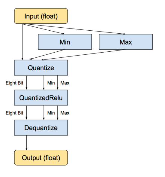
The min and max operations actually look at the values in the input float tensor, and then feeds them into the Dequantize operation that converts the tensor into eight-bits. There’s more details on how the quantized representation works later on.

Once the individual operations have been converted, the next stage is to remove unnecessary conversions to and from float. If there are consecutive sequences of operations that all have float equivalents, then there will be a lot of adjacent Dequantize/Quantize ops. This stage spots that pattern, recognizes that they cancel each other out, and removes them, like this:

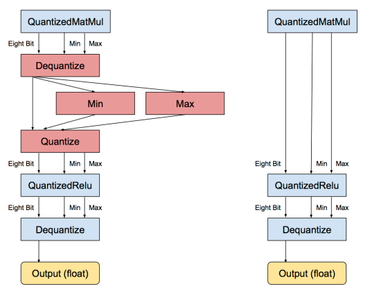
Applied on a large scale to models where all of the operations have quantized equivalents, this gives a graph where all of the tensor calculations are done in eight bit, without having to convert to float.

What Representation is Used for Quantized Tensors?

We approach converting floating-point arrays of numbers into eight-bit representations as a compression problem. We know that the weights and activation tensors in trained neural network models tend to have values that are distributed across comparatively small ranges (for example you might have -15 to +15 for weights, -500 to 1000 for activations on an image model, though the exact numbers will vary). We also know from experiment that neural nets tend to be very robust in the face of noise, and so the noise-like error produced by quantizing down to a small set of values will not hurt the precision of the overall results very much. We also want to pick a representation that’s easy to perform calculations on, especially the large matrix multiplications that form the bulk of the work that’s needed to run a model.

These led us to pick a representation that has two floats to store the overall minimum and maximum values that are represented by the lowest and highest quantized value. Each entry in the quantized array represents a float value in that range, distributed linearly between the minimum and maximum. For example, if we have minimum = -10.0, and maximum = 30.0f, and an eight-bit array, here’s what the quantized values represent:

Quantized | Float
----------+-----
   0      | -10.0
 255      |  30.0
 128      |  10.0

The advantages of this format are that it can represent arbitrary magnitudes of ranges, they don’t have to be symmetrical, it can represent signed and unsigned values, and the linear spread makes doing multiplications straightforward. There are alternatives like Song Han’s code books that can use lower bit depths by non-linearly distributing the float values across the representation, but these tend to be more expensive to calculate on.

The advantage of having a strong and clear definition of the quantized format is that it’s always possible to convert back and forth from float for operations that aren’t quantization-ready, or to inspect the tensors for debugging purposes. One implementation detail in TensorFlow that we’re hoping to improve in the future is that the minimum and maximum float values need to be passed as separate tensors to the one holding the quantized values, so graphs can get a bit dense!

How do we Determine Ranges?

The nice thing about the minimum and maximum ranges is that they can often be pre-calculated. Weight parameters are constants known at load time, so their ranges can also be stored as constants. We often know the ranges for inputs (for examples images are usually RGB values in the range 0.0 to 255.0), and many activation functions have known ranges too. This can avoid having to analyze the outputs of an operation to determine the range, which we need to do for math ops like convolution or matrix multiplication which produce 32-bit accumulated results from 8-bit inputs.

If you’re doing any kind of arithmetic on 8-bit inputs, you’ll naturally start to accumulate results that have more than 8 bits of precision. If you add two 8 bit values, the result needs 9 bits. If you multiply two 8 bit numbers, you get 16 bits in the output. If you total up a series of 8-bit multiplications, like we do for matrix multiplication, the results grow beyond 16 bits, with the accumulator typically needing at least 20 to 25 bits, depending on how long the dot products involved are.

This can be an issue for our quantization approach, since we need to take an output that’s much wider than 8 bits and shrink it down to feed into the next operation. One way to do it for matrix multiplies would be to calculate the largest and smallest possible output values, assuming all of the input values were at extremes. This is safe, since we know mathematically that no results can fall outside this range, but in practice most weights and activation values are much more evenly distributed. This means that the actual range of values we see is much smaller than the theoretical one, so if we used the larger bounds we’d be wasting a lot of our 8 bits on numbers that never appeared. Instead, we use the QuantizeDownAndShrinkRange operator to take a 32-bit accumulated tensor, analyze it to understand the actual ranges used, and rescale so that the 8-bit output tensor uses that range effectively. There are strategies that involve observing the actual minimums and maximums encountered with large sets of training data, and hard-coding those to avoid analyzing the buffer for ranges every time, but we don’t currently include that optimization.

How is the Rounding Done?

One of the hardest and most subtle problems we hit during quantization was the accumulation of biases. As I mentioned above, neural networks are very resilient to noise, but unless you’re very careful with rounding it’s easy to introduce biases in a single direction that build up during computation and wreck the final accuracy. You can see the final formula in the code, but the important part was that we needed to subtract the rounded version of the minimum from the rounded version of the float input value, rather than subtracting float minimum from the input and then rounding.

What’s Next?

We’ve found that we can get extremely good performance on mobile and embedded devices by using eight-bit arithmetic rather than floating-point. You can see the framework we use to optimize matrix multiplications at gemmlowp. We still need to apply all the lessons we’ve learned to the TensorFlow ops to get maximum performance on mobile, but we’re actively working on that. Right now, this quantized implementation is a reasonably fast and accurate reference implementation that we’re hoping will enable wider support for our eight-bit models on a wider variety of devices.

If you’re interested, I highly recommend digging through the quantization code in TensorFlow, especially looking at the kernels that implement quantized ops. These all include reference implementations that we’re hoping will help portability to new hardware devices.

We also hope that this demonstration will encourage the community to explore what’s possible with low-precision neural networks. Thanks to everyone who helped put the quantization support together, it’s been great getting this out there!