When I was first learning programming in the 90’s, embedded systems were completely out of reach. I couldn’t afford the commercial development boards and toolchains that I’d need to even get started, and I’d need a lot of proprietary knowledge just to get started. I was excited a few years ago when the Arduino environment first appeared, since it removed a lot of the barriers to the general public. I still didn’t dive in though, because I couldn’t see an easy way to port the kind of algorithms I was interested in to eight-bit hardware, and even the coding environment wasn’t a good fit for my C++ background.
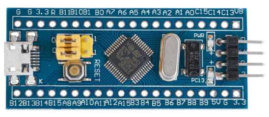
That’s why I’ve been fascinated by the rise of the ARM M-series chips. They’re cheap, going for as little as $2 for a “blue pill” M3 board on ebay, they can run with very low power usage which can be less than a milliwatt (offering the chance to run on batteries for months or years), and they have the full 32-bit ARM instruction I’m familiar with. This makes them tempting as a platform to prototype the kind of smart sensors I believe the combination of deep learning eating software and cheap, low-power compute power is going to enable.
I was still daunted by the idea of developing for them though. Raspberry Pi’s are very approachable because you can use a very familiar Linux environment to program them, but there wasn’t anything as obvious for me to use in the M-series world. Happily I was able to get advice from some experts at ARM, who helped steer me as a newbie through this unfamiliar world. I was very pleasantly surprised by the maturity and ease of use of the development ecosystem, so I want to share what I learned for anyone else who’s interested.
The first tip they had was to check out STMicroelectronics “Discovery” boards. These are small circuit boards with an M-series CPU and often a lot of peripherals built in to make experimentation easy. I started with the 32F746G which included a touch screen, audio input and output, microphones, and even ethernet, and cost about $70. There are cheaper versions available too, but I wanted something easy to demo with. I also chose the M7 chip because it has support for floating point calculations, even though I don’t expect I’ll need that long term it’s helpful when porting and prototyping to have it.
The unboxing experience was great, I just plugged the board into a USB socket on my MacBook Pro and it powered itself up into some demonstration programs. It showed up on my MacOS file system as a removable drive, and the usefulness of that quickly became clear when I went to the mbed online IDE. This is one of the neatest developer environments I’ve run across, it runs completely in the browser and makes it easy to clone and modify examples. You can pick your device, grab a project, press the compile button and in a few seconds you’ll have a “.bin” file downloaded. Just drag and drop that from your downloads folder into the USB device in the Finder and the board will reboot and run the program you’ve just built.
I liked this approach a lot as a way to get started, but I wasn’t sure how to integrate larger projects into the IDE. I thought I’d have to do some kind of online import, and then keep copies of my web code in sync with more traditional github and file system versions. When I was checking out the awesome keyword spotting code from ARM research I saw they were using a tool called “mbed-cli“, which sounded a lot easier to integrate into my workflow. When I’m doing a lot of cross platform work, I usually find it easier to use Emacs as my editor, and a custom IDE can actually get in the way. As it turns out, mbed-cli offers a command line experience while still keeping a lot of the usability advantages I’d discovered in the web IDE. Adding libraries and aiming at devices is easy, but it integrates smoothly with my local file system and github. Here’s what I did to get started with it:
- I used
pip install mbed-clion my MacOS machine to add the Python tools to my system. - I ran
mbed new mbed-hello-worldto create a new project folder, which the mbed tools populated with all the baseline files I needed, and then I cd-ed into it withcd mbed-hello-world - I decided to use gcc for consistency with other platforms, so I downloaded the GCC v7 toolchain from ARM, and set a global variable to point to it by running
mbed config -G GCC_ARM_PATH "/Users/petewarden/projects/arm-compilers/gcc-arm-none-eabi-7-2017-q4-major/bin" - I then added a ‘main.cpp’ file to my empty project, by writing out this code:
#include <mbed.h>

Serial pc(USBTX, USBRX);

int main(int argc, char** argv) {
  pc.printf("Hello world!\r\n");
  return 0;
}
The main thing to notice here is that we don’t have a natural place to view stdout results from a normal printf on an embedded system, so what I’m doing here is creating an object that can send text over a USB port using an API exported from the main mbed framework, and then doing a printf call on that object. In a later step we’ll set up something on the laptop side to display that. You can see the full mbed documentation on using printf for debugging here.
- I did
git add main.cppandgit commit -a "Added main.cpp"to make sure the file was part of the project. - I created a new terminal window to look at the output of the printf after it’s been sent over the USB connection. How to view this varies for different platforms, but for MacOS you need to enter the command
screen /dev/tty.usbm, and press Tab to autocomplete the correct device name. After that, the terminal may contain some random text, but after you’ve successfully compiled and run the program you should see “Hello World!” output. One quirk I noticed was that\non its own was not enough to cause the normal behavior I expected from a new line, in that it just moved down one line but the next output started at the same horizontal position. That’s why I added a\rcarriage return character in the example above. - I ran
mbed compile -m auto -t GCC_ARM -fto build and flash the resulting ‘.bin’ file onto the Discovery board I had plugged in to the USB port. The-m autopart made the compile process auto-discover what device it should be targeting, based on what was plugged in, and-ftriggered the transfer of the program after a successful build. - If it built and ran correctly, you should see “Hello World!” in the terminal window where you’re running your screen command.
I’ve added my version of this project on Github as github.com/petewarden/mbed-hello-world, in case you want to compare with what you get following these steps. I found the README for the mbed-cli project extremely clear though, and it’s what most of this post is based on.
My end goal is to set up a simple way to compile a code base that’s shared with other platforms for M-series devices. I’m not quite certain how to do that (for example integrating with a makefile, or otherwise syncing a list of files between an mbed project and other build systems), but so far mbed has been such a pleasant experience I’m hopeful I’ll be able to figure that out soon!


 Photo by oatsy40