An engineer who’s learning about using convolutional neural networks for image classification just asked me an interesting question; how does a model know how to recognize objects in different positions in an image? Since this actually requires quite a lot of explanation, I decided to write up my notes here in case they help some other people too.

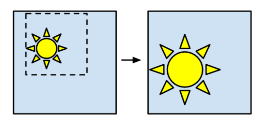
Here’s two example images showing the problem that my friend was referring to:

If you’re trying to recognize all images with the sun shape in them, how do you make sure that the model works even if the sun can be at any position in the image? It’s an interesting problem because there are really three stages of enlightenment in how you perceive it:

• If you haven’t tried to program computers, it looks simple to solve because our eyes and brain have no problem dealing with the differences in positioning.
• If you have tried to solve similar problems with traditional programming, your heart will probably sink because you’ll know both how hard dealing with input differences will be, and how tough it can be to explain to your clients why it’s so tricky.
• As a certified Deep Learning Guru, you’ll sagely stroke your beard and smile, safe in the knowledge that your networks will take such trivial issues in their stride.

My friend is at the third stage of enlightenment, but is smart enough to realize that there are few accessible explanations of why CNNs cope so well. I don’t claim to have any novel insights myself, but over the last few years of working with image models I have picked up some ideas from experience, and heard folklore passed down through the academic family tree, so I want to share what I know. I would welcome links to good papers on this, since I’m basing a lot of this on hand-wavey engineering intuition, so please do help me improve the explanation!

The starting point for understanding this problem is that networks aren’t naturally immune to positioning issues. I first ran across this when I took networks trained on the ImageNet collection of photos, and ran them on phones. The history of ImageNet itself is fascinating. Originally, Google Image Search was used to find candidate images from the public web by searching for each class name, and then researchers went through the candidates to weed out any that were incorrect. My friend Tom White has been having fun digging through the resulting data for anomalies, and found some fascinating oddities like a large number of female models showing up in the garbage truck category! You should also check out Andrej Karpathy’s account of trying to label ImageNet pictures by hand to understand more about its characteristics.

The point for our purposes is that all the images in the training set are taken by people and published on websites that rank well in web searches. That means they tend to be more professional than a random snapshot, and in particular they usually have the subject of the image well-framed, near the center, taken from a horizontal angle, and taking up a lot of the picture. By contrast, somebody pointing a phone’s live camera at an object to try out a classifier is more likely to be at an odd angle, maybe from above, and may only have part of the object in frame. This meant that models trained on ImageNet had much worse perceived performance when running on phones than the published accuracy statistics would suggest, because the training data was so different than what they were given by users. You can still see this for yourself if you install the TensorFlow Classify application on Android. It isn’t bad enough to make the model useless on mobile phones, since there’s still usually some framing by users, but it’s a much more serious problem on robots and similar devices. Since their camera positioning is completely arbitrary, ImageNet-trained models will often struggle seriously. I usually recommend developers of those applications look out for their own training sets captured on similar devices, since there are also often other differences like fisheye lenses.

Even still, within ImageNet there is still a lot of variance in positioning, so how do networks cope so well? Part of the secret is that training often includes adding artificial offsets to the inputs, so that the network has to learn to cope with these differences.

Before each image is fed into the network, it can be randomly cropped. Because all inputs are squashed to a standard size (often around 200×200 or 300×300), this has the effect of randomizing the positioning and scale of objects within each picture, as well as potentially cutting off sections of them. The network is still punished or rewarded for its answers, so to get good performance it has to be able to guess correctly despite these differences. This explains why networks learn to cope with positioning changes, but not how.

To delve into that, I have to dip into a bit of folklore and analogy. I don’t have research to back up what I’m going to offer as an explanation, but in my experiments and discussions with other practitioners, it seems pretty well accepted as a working theory.

Ever since the seminal AlexNet, CNN’s have been organized as consecutive layers feeding data through to a final classification operation. We think about the initial layers as being edge detectors, looking for very basic pixel patterns, and then each subsequent layer takes those as inputs and guesses higher and higher level concepts as you go deeper. You can see this most easily if you view the filters for the first layer of a typical network:

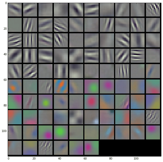
Image by Evan Shelhamer from Caffenet

What this shows are the small patterns that each filter is looking for. Some of them are edges in different orientations, others are colors or corners. Unfortunately we can’t visualize later layers nearly as simply, though Jason Yosinski and others have some great resources if you do want to explore that topic more.

Here’s a diagram to try to explain the concepts involved:

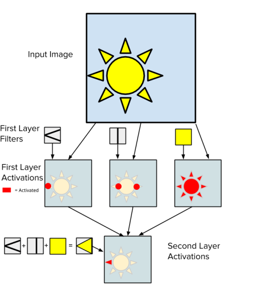
What it’s trying to show is that the first layer is looking for very simple pixel patterns in the image, like horizontal edges, corners, or patches of solid color. These are similar to the filters shown in the CaffeNet illustration just above. As these are run across the input image, they output a heat map highlighting where each pattern matches.

The tricky bit to understand is what happens in the second layer. The heatmap for each simple filter in the first layer is put into a separate channel in the activation layer, so the input to the second layer typically has over a hundred channels, unlike the three or four in a typical image. What the second layer is looking for is more complex patterns in these heatmaps combined together. In the diagram we’re trying to recognize one petal of the sun. We know that this has a sharp corner on one end, and nearby will be a vertical line, and the center will be filled with yellow. Each one of these individual characteristics is represented by one channel in the input activation layer, and the second layer’s filter for “petal facing left” looks for parts of the images where all three occur together. In areas of the image where only one or two are present, nothing is output, but where all three are there the output of the second layer will show high activation.

Just like with the first layer, there are many filters in the second layer, and you can think of each one as representing a higher-level concept like “petal facing up”, “petal facing right”, and others. This is harder to visualize, but results in an activation layer with many channels, each representing one of those concepts.

As you go deeper into the network, the concepts get higher and higher level. For example, the third or fourth layer here might activate yellow circles surrounded by petals, by combining the relevant input channels. From that representation it’s fairly easy to write a simple classifier that spots whenever a sun is present. Of course real-world classifiers don’t represent concepts nearly as cleanly as I’ve laid out above, since they learn how to break down the problem themselves rather than being supplied with human-friendly components, but the same basic ideas hold.

This doesn’t explain how the network deals with position differences though. To understand that, you need to know about another common design trait of CNNs for image classification. As you go deeper into a network, the number of channels will typically increase, but the size of the image will shrink. This shrinking is done using pooling layers, traditionally with average pooling but more commonly using maximum pooling these days. Either way, the effect is pretty similar.

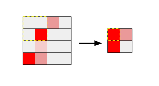
Here you can see that we take an image and shrink it in half. For each output pixel, we look at a 2×2 input patch and choose the maximum value, hence the name maximum pooling. For average pooling, we take the mean of the four values instead.

This sort of pooling is applied repeatedly as values travel through the network. This means that by the end, the image size may have shrunk from 300×300 to 13×13. This shrinkage also means that the number of position variations that are possible has shrunk a lot. In terms of the example above, there are only 13 possible horizontal rows for a sun image to appear in, and only 13 vertical columns. Any smaller position differences are hidden because the activations will be merged into the same cell thanks to max pooling. This makes the problem of dealing with positional differences much more manageable for the final classifier, since it only has to deal with a much simpler representation than the original image.

This is my explanation for how image classifiers typically handle position changes, but what about similar problems like offsets in audio? I’ve been intrigued by the recent rise of “dilated” or “atrous” convolutions that offer an alternative to pooling. Just like max pooling, these produce a smaller output image, but they do it within the context of the convolution itself. Rather than sampling adjacent input pixels, they look at samples separated by a stride, which can potentially be quite large. This gives them the ability to pull non-local information into a manageable form quite quickly, and are part of the magic of DeepMind’s WaveNet paper, giving them the ability to tackle a time-based problem using convolution rather than recurrent neural networks.

I’m excited by this because RNNs are a pain to accelerate. If you’re dealing with a batch size of one, as is typical with real-time applications, then most of the compute is matrix time vector multiplications, with the equivalent of fully-connected layers. Since every weight is only used once, the calculations are memory bound rather than compute bound as is typically the case with convolutions. Hence I have my fingers crossed that this becomes more common in other domains!

Anyway, thanks for making it this far. I hope the explanation is helpful, and I look forward to hearing ideas on improving it in the comments or on twitter.