A colleague recently asked for more details on an approach I recommended, but which she hadn’t seen any documentation for. I realized that it was something I’d learned from talking to model builders at Google, and I wasn’t sure there was anything written up, so in the spirit of leaving a trail of breadcrumbs for anyone coming after, I thought I should put it into a quick blog post.
The summary is that if you have MaxPool or AveragePool after a convolutional layer in a network, and you’re targeting a resource-constrained system like a microcontroller, you should try removing them entirely and replacing them with a stride in the convolution instead. This has two main benefits, but to explain it’s easiest to diagram out the network before and after.

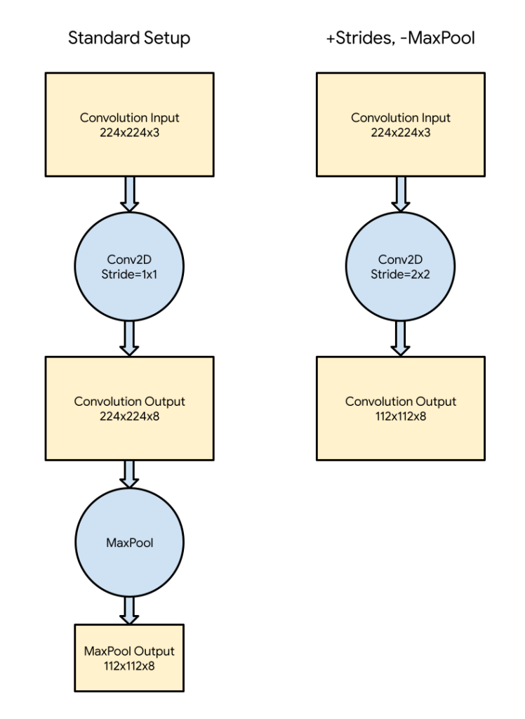
In the typical setup, shown on the left, is a convolutional layer is followed by a pooling operation. This has been common since at least AlexNet, and is still found in many modern networks. The setup I often find useful is shown on the right. I’m using an example input size of 224 wide by 224 high for this diagram, but the discussion holds true for any dimensions.
The first thing to notice is that in the standard configuration, there’s a 224x224x8 activation buffer written out to memory after the convolution layer. This is by far the biggest chunk of memory required in this part of the graph, taking over 400KB, even with eight-bit values. All ML frameworks I’m aware of will require this buffer to be instantiated and filled before the next operation can be invoked. In theory it might be possible to do tiled execution, in the way that’s common for image processing frameworks, but the added complexity hasn’t made it a priority so far. If you’re running on an embedded system, 400KB is a lot of RAM, especially since it’s only being used for temporary values. That makes it a tempting target for size optimization.
My second observation is that we’re only using 25% of those values, assuming MaxPool is doing a typical 2x reduction, taking the largest value out of 4 in a 2×2 window. From experience, these values are often very similar, so while doing the pooling does help overall accuracy a bit, taking any of those four values at random isn’t much worse. In essence, this is what removing the pooling and increasing the stride for convolution does.
Stride is an argument that controls the step size as a convolution filter is slid across the input. By default, many networks have windows that are offset from each other by one pixel horizontally, and one pixel vertically. This means (ignoring padding, which is a whole different discussion) the output is the same size as the input, but typically with more channels (eight in the diagram above). Instead of setting the stride to this default of 1 horizontally, 1 vertically, you can set it to 2,2. This means that each window is offset by two pixels vertically and horizontally from its neighbor. This results in an output array that is half the width and height of the input, and so has a quarter of the number of elements. In essence, we’re picking one of the four values that would have been chosen by the pooling operation, but without the comparison or averaging that is used in the standard configuration.
This means that the output of the convolution layer uses much less memory, resulting in a smaller arena for TFL Micro, but also reduces the computation by 75%, since only a quarter of the convolution windows are being calculated. It does result in some accuracy loss, which you can verify during training, but since it reduces the resource usage so dramatically you may even be able to increase some other parameters like the input size or number of channels and gain some back. If you do find yourself struggling for arena size, I highly recommend giving this approach a try, it’s been very helpful for a lot of our models. If you’re not sure if your model has the convolution/pooling pattern, or want to better understand the sizes of your activation buffers and how they influence the arena you’ll need, I recommend the Netron visualizer, which can take TensorFlow Lite model files.
Pingback: Shrinking Convolutional Neural Networks for TinyML – Curated SQL
From a (multi-rate) signal processing perspective, all of these setups (with MaxPool, with AveragePool, striding) are methods of down-sampling. Striding corresponds to the simplest possible approach of decimation, i.e. just (logically) sample the output at the lower rate.
Trading latency for space, one could perform these decimated convolutions multiple times with different offsets sequentially accumulating the results with max/average to get the original result with less intermediate space usage. This could be viewed as a kind of “tiling in frequency-phase space”. One could pick various points between the fully decimated output and the fully reconstructed output to trade off “accuracy” for space and latency. Similarly, one could pick different numbers to execute in parallel to trade off latency for space. (Of course, if you pick maximum parallelization with maximum reconstruction, you just end up manually parallelizing the original Conv2D, which presumably Conv2D already did and better.)